
Real time object detection using YOLO or SSD
- Aryan Parikh
- Nov 30, 2025
- 11 min read
Contents
Introduction
Modern AI doesn’t just see images – it understands them.It can tell you there’s a dog in your photo, sure, but it can also say:“There’s a dog here, a person there, and a car behind them.”
That ability to both recognise and locate objects is called object detection.
Two highly influential and widely used real-time object detectors are:
YOLO (You Only Look Once)
SSD (Single Shot MultiBox Detector)
These models are built on top of convolutional neural networks (CNNs) like the one you described in your example article. They use convolution layers, pooling layers and fully connected layers — but they arrange and extend them in clever ways so that, in a single pass, they can output multiple bounding boxes and class predictions.
In this article, we’ll walk through:
what object detection actually is,
how it extends basic image classification,
how YOLO and SSD work under the hood (at an intuitive level),
and where they’re used in real life.
By the end, you should feel as comfortable talking about YOLO and SSD as you do about basic CNN architecture.
What Is Object Detection?
At its core, object detection solves two problems at the same time:
What is present in the image? → Classification
Where is it located? → Localization
The model doesn’t just say: “This is an image of a cat.”
Instead, it produces something like:
Class: car
Bounding box: (x, y, width, height)

And often not just one of these, but many — one for each object in the image.You can think of it as attaching a labelled rectangle around every relevant object in the scene.
From Image Classification to Object Detection
Let’s briefly recall what a standard CNN classifier does.
You feed it an image, it passes through:
Convolution + pooling layers → extract features
Fully connected layers → combine features
Softmax output → probability for each class
For image classification, the output is usually a single label:
dog (with 0.97 probability, for example)
But images in the real world are rarely that simple:
A street scene: cars, people, traffic lights, bicycles
A kitchen: plates, cups, microwave, fridge
A medical scan: multiple lesions or anomalies
If you only use a classifier, you get one label for the entire image. You don’t know:
how many objects are present,
where they are,
or which pixels belong to which object.
This is where object detection architectures, such as YOLO and SSD, come in. They extend the basic CNN idea so that the output isn’t just one label, but a set of boxes plus labels.
Bounding Boxes, Confidence Scores and IoU
Before diving into YOLO and SSD, let’s clarify a few core concepts.
Bounding Box
A bounding box is usually represented by four numbers. Common parameterisations are:
(x_min, y_min, x_max, y_max) — corners
(x_center, y_center, width, height) — centre + size
These values are often normalised by the image width and height (so they’re between 0 and 1).

Confidence Score(Objectness)
Each predicted box comes with a confidence score, which answers:
“How sure is the model that this box actually contains an object?”
Higher confidence → more likely to be a real object.Often, there is also a probability distribution over classes (dog, cat, person, etc.), so you can think of each detection as:
Box
Objectness (is there any object?)
Class probabilities
Intersection over Union (IoU)
How do we know if a predicted box matches the ground-truth box?
We use IoU — Intersection over Union.
Imagine two rectangles:
One is the ground truth (human-annotated).
The other is the prediction.
IoU is calculated as:
IoU = (Area of Overlap) / (Area of Union)
IoU = 1 → perfect overlap
IoU = 0 → no overlap at all
IoU > 0.5 (often used as a threshold) → considered a “good” match
IoU is crucial during training (to compute loss) and during post-processing (to merge duplicate predictions).
The General Object Detection Pipeline
Almost all modern object detectors — including YOLO and SSD — share a common high-level structure:
Feature Extraction
A CNN (like VGG, ResNet, or a custom backbone) processes the image and extracts feature maps.
Bounding Box & Class Prediction
On top of the features, special layers predict many candidate bounding boxes and their class scores.
Filtering & Post-Processing
Low-confidence boxes are removed.
Overlapping boxes are merged using Non-Max Suppression.
YOLO and SSD differ mostly in how they organise step 2 (prediction) and how they decide where to look for objects.
YOLO (You Only Look Once)
YOLO’s main philosophy is in its name:
You Only Look Once – the network looks at the image a single time and simultaneously predicts all bounding boxes and class probabilities.
It treats detection as a single regression problem: from image pixels directly to bounding box coordinates and class labels.
Intuition
Traditional detectors before YOLO often used a two-step process:
Propose candidate regions (region proposals).
Run a classifier on each region
This is computationally expensive and not ideal for real-time use.YOLO discards region proposals and instead says:
“Let’s take the whole image, run it through a CNN once, and directly output everything we need.”
This makes YOLO extremely fast and relatively simple conceptually.
Grid Cells and Predictions
YOLO divides the input image into an S × S grid.
Each grid cell is responsible for detecting objects whose center falls inside that cell.Think of it like placing a chessboard over the image.

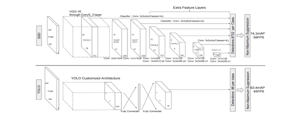
This diagram illustrates the YOLO v1 detection pipeline. A 448×448 RGB image is first passed through YOLO’s custom Darknet feature extractor, which processes the image using convolution and pooling layers to produce a 7×7×1024 feature map. This map is flattened and fed through two fully connected layers, generating a final 7×7×30 output tensor. Each of the 49 grid cells predicts 2 bounding boxes (5 values each: x, y, w, h, objectness) and 20 class probabilities, giving 30 values per cell. Altogether, YOLO outputs 98 candidate boxes, which are filtered using non-maximum suppression to remove duplicates and keep only the strongest predictions. This architecture enables YOLO v1 to achieve real-time performance at 45 FPS with 63.4% mAP on Pascal VOC.
Each square:
looks at the underlying part of the image,
guesses if there’s an object center inside,
and if so, predicts bounding box(es) and class probabilities.
For each grid cell, YOLO typically predicts:
B bounding boxes, each with:
x, y, w, h (bounding box)
objectness score (how likely it is that an object exists in that box)
C class probabilities (one for each class in the dataset)
So the total output per grid cell combines both where and what.The x and y coordinates are usually relative to the top-left corner of the grid cell. This constrains the model so that predictions remain spatially reasonable.
Anchor Boxes
In early YOLO versions, each grid cell predicted a fixed number of boxes directly. Later versions (like YOLOv2 onwards) introduced anchor boxes (similar to SSD’s default boxes).
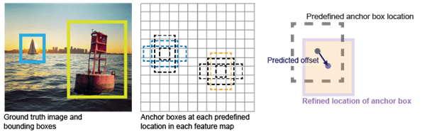
Anchor boxes are predefined shapes (aspect ratios and scales) associated with each grid cell.
Why?
Objects in images come in different shapes:
Tall and thin (person)
Short and wide (car, bus)
Almost square (some animals, faces)
If the model always starts from a generic box, it may struggle to cover all shapes efficiently. By giving it several anchor boxes, each cell can adjust (or “refine”) the box that best matches the object.
During training, ground truth boxes are assigned to the most appropriate anchor boxes based on IoU. The model then learns offsets from the anchor box to the ground truth box.
How YOLO Learns
At a high level, YOLO’s training loss is composed of three main ideas:
Localization Loss
Measures how far the predicted box (x, y, w, h) is from the ground truth box.
Confidence/Objectness Loss
Encourages high scores for boxes that contain objects.
Penalises boxes that predict high confidence but don’t match any object.
Classification Loss
Encourages accurate class predictions for each box that corresponds to an object.
Put together, the network learns to:
put boxes in the right places,
be honest about when a box is “real”
and correctly classify the content of each box.
The beauty is that all of this is learned simultaneously in one end-to-end network.
Non-Max Suppression (NMS) in YOLO
Because each grid cell predicts multiple boxes and many may overlap heavily, the raw output has a lot of candidate boxes.
We don’t want to show 10 slightly different boxes all around the same dog.

Non-Max Suppression (NMS) removes redundant boxes.
The general NMS procedure is:
Filter out boxes with very low confidence scores.
Among the remaining boxes, pick the one with the highest confidence.
Remove all boxes that have a high IoU (e.g., > 0.5) with this box.
Repeat with the next highest-confidence box.
After NMS, we’re left with a small, clean set of boxes, each ideally corresponding to a distinct object.
SSD (Single Shot MultiBox Detector)
SSD shares YOLO’s goal: real-time object detection in a single forward pass.But SSD approaches the problem a bit differently, focusing heavily on multi-scale detection — that is, detecting objects of different sizes using different layers of the network.
One key intuition: Earlier layers in a CNN have higher spatial resolution and are better for detecting small objects. Deeper layers have coarser resolution but more semantic information, which helps detect larger, more complex objects.
SSD takes advantage of this by performing detection on multiple feature maps at different resolutions.
Intuition
Think of SSD as:
A base CNN (like VGG or MobileNet) that extracts general image features.
A series of extra convolutional layers that progressively reduce spatial dimensions.
At each of these layers, SSD places small “heads” that predict bounding boxes and class scores.

So instead of a single grid as in YOLO, SSD effectively uses several grids, each on a different feature map scale.
Multi-Scale Feature Maps
Let’s assume SSD uses several feature maps (for example):
38 × 38
19 × 19
10 × 10
5 × 5
3 × 3
1 × 1
Each of these feature maps corresponds to a different receptive field size:
The 38 × 38 map sees fine details → good for small objects.
The 1 × 1 map sees the entire image → good for very large objects.
On each feature map, SSD applies a small convolutional filter that, for each cell, predicts:
offsets for several bounding boxes,
confidence scores,
and class probabilities.
This multi-scale prediction mechanism allows SSD to naturally cover a wide range of object sizes.
Default (Prior) Boxes
Just like anchor boxes in YOLO, SSD uses default boxes (also called prior boxes) at each feature map location.
Each location on a feature map comes with several default boxes of different:
scales (small, medium, large relative to that map),
aspect ratios (1:1, 2:1, 1:2, etc.).
During training, SSD matches each ground truth box to the default box with the highest IoU (and sometimes to additional default boxes with IoU above a threshold).
Then, the model learns to:
adjust the default box (shift, scale) to match the ground truth (localization),
and predict the right class label (classification).
This design is very flexible and dense: SSD can place many potential boxes across many feature maps.
How SSD Learns
The training objective for SSD also combines multiple components:
Localization Loss
Measures the error between predicted box offsets and ground truth boxes (only for default boxes matched to a real object).
Confidence Loss
Encourages correct classification of each default box as either “background” or one of the object classes.
Hard Negative Mining
Because there are many more default boxes than actual objects, most default boxes are background.
SSD uses a technique called hard negative mining to focus on the background boxes that the model is currently getting wrong, rather than all of them.
The combined loss pushes SSD to learn:
where to adjust default boxes,
when to say “this is background, nothing here,”
and when to confidently declare an object and its class.
As with YOLO, SSD is trained end-to-end.
YOLO vs SSD – A Side-by-Side Comparison
Let’s compare YOLO and SSD along several dimensions.
1. Architecture Style
YOLOA single grid over the image.
Predictions are tied strongly to grid cells.
Anchor boxes added in later versions.
SSD
Multiple feature maps at different resolutions.
Default boxes at each location of each map.
Particularly strong at handling objects of different scales.
2. Speed
Both are designed for real-time detection, but exact speed depends on:
model version,
input size,
hardware,
and implementation.
Historically:
YOLO was often slightly faster at similar accuracy targets.
SSD was very competitive, especially with lightweight backbones like MobileNet (SSD-MobileNet).
3. Small Object Detection
YOLO (especially early versions) sometimes struggles more with small objects because of the coarse grid representation.
SSD often performs better on small objects thanks to its high-resolution feature maps (e.g., the 38×38 map).
4. Implementation Complexity
Both are relatively straightforward to use via modern libraries and frameworks.
Conceptually, SSD’s multi-scale feature maps and default boxes add some complexity, but the underlying principles are similar (anchor-based regression + classification).
5. Use Cases
YOLO
Real-time detection on video streams.
Robotics and drones (limited compute, need fast inference).
Applications where speed is more critical than squeezing out every bit of accuracy.
SSD
Mobile and embedded devices (SSD + MobileNet).
Scenarios that benefit from multi-scale detection.
Where Are YOLO and SSD Used?
You’ll find YOLO and SSD (or their variants) in many real-world applications, such as:
Self-driving cars
Detecting pedestrians, other vehicles, traffic signs and traffic lights.
Surveillance systems
Detecting intruders, unattended objects or suspicious activity.
Retail analytics
Counting customers, tracking product placement, analysing shelf usage.
Robotics and drones
Avoiding obstacles, locating targets, interacting with objects.
Medical imaging
Detecting lesions, tumours, organs of interest in scans (when adapted and fine-tuned).
In many modern systems, these models are further combined with tracking, segmentation, or RAG-style pipelines to form complex, intelligent applications.
Common Challenges in Object Detection
Although YOLO and SSD are powerful, object detection is far from trivial. Some challenges include:
1. Small and Distant Objects
Objects that occupy only a few pixels are difficult to detect reliably. Multi-scale feature maps (SSD) and more advanced architectures help, but it remains a challenging problem.
2. Occlusion and Clutter
If objects overlap or are partially hidden (e.g., one person standing behind another), predictions become more uncertain. Correctly assigning bounding boxes to partially visible objects is hard.
3. Class Imbalance
Some object categories appear far more often than others (e.g., “person” vs. “traffic light”). Models can become biased toward frequent classes. Loss functions and sampling strategies (like hard negative mining) help mitigate this.
4. Real-Time Constraints
In safety-critical applications (self-driving, robotics), detection must be not just accurate but consistently fast, even on limited hardware. This drives ongoing research into lighter, more efficient variants of YOLO and SSD.
Summary
In this article, we explored object detection and two of its most influential architectures: YOLO and SSD.
We began by understanding the difference between classification and detection:
Classification tells us what is in an image.
Detection tells us what and where.
We then introduced key concepts:
Bounding boxes — the rectangles used to localise objects.
Confidence scores — how sure the model is.
IoU (Intersection over Union) — the metric for overlap between predictions and ground truth.
Next, we looked at:
YOLO:
Divides the image into a grid.
Each cell predicts bounding boxes and class probabilities.
Uses anchor boxes, a combined loss, and non-max suppression to produce final detections.
SSD:
Builds on a base CNN with additional layers.
Uses multi-scale feature maps to detect both small and large objects.
Uses default boxes (prior boxes) at each location and learns offsets and class labels.
We compared YOLO and SSD along speed, architecture, and performance on different object sizes, and we briefly discussed where they are used, as well as some real-world challenges.
Just as convolutional, pooling and fully connected layers combine to form a CNN classifier, these same building blocks, when arranged in more sophisticated ways, give us powerful object detectors like YOLO and SSD.
If you’ve reached this far, you now have a solid conceptual understanding of how real-time object detection works — more than enough to write a detailed blog in the same style as your CNN article.


Comments